SINDy
Implementing the SINDy algorithm in PETSc.
The code is in the PETSc repo here.
Mathematical theory
This discussion is based on Brunton et al. (2016) and Shea et al. (2020). I’m going to try to outline the general case. \[\begin{align} \mathbf{u} &= \mathbf{u}(\mathbf{x}, t) \\ \frac{d\mathbf{u}}{dt} &= \frac{d\mathbf{u}}{dt}(\mathbf{u}, \mathbf{x}, t) \end{align}\] for \(\mathbf{u} \in \mathbb{R}^{d_u}, \,\, \mathbf{x} \in \mathbb{R}^{d_x}, \,\, t \in \mathbb{R}\). The goal of SINDy is to represent \(\frac{d\mathbf{u}}{dt}\) in a basis \(B\) of size \(p\) with sparse coefficients \(\mathbf{c} \in \mathbb{R}^p\). \[\begin{equation} \frac{d\mathbf{u}}{dt} \approx \sum_{i=1}^p c_i \mathbf{b_i}(\mathbf{u},\mathbf{x},t) \end{equation} \tag{1}\] \[\begin{align} b_i \in B = \{\mathbf{1}, \mathbf{u}, \mathbf{x}, t, \mathbf{u}^2, \mathbf{u}\mathbf{x},\mathbf{u}t,\mathbf{x}^2,\mathbf{x}t,t^2,\ldots,\sin\mathbf{u},\cos{\mathbf{u}}, \frac{\partial\mathbf{u}}{\partial \mathbf{x}},\ldots\} \end{align}\] This will generally be represented as a linear system with discretized \(\mathbf{U}\) and \(\mathbf{X}\), with the columns of the matrix \(\Theta\) represented basis functions evaluated at specific \(\mathbf{X}\) and \(t\). \[\begin{equation} \frac{d\mathbf{U}}{dt} \approx \Theta(\mathbf{U}, \mathbf{X}, t) \mathbf{c} \end{equation} \tag{2}\]
Note that when \(d_x \ne 1\) or \(d_u \ne 1\), the vector terms in the basis shown above aren’t mathematically well-defined, but the idea is to include polynomial terms, and these can also include polynomial terms of separate components of the vector, and cross terms of those components. The functions shown in the basis above are just examples; the main idea is that the basis can have any kind of functions of \(\mathbf{u}\), \(\mathbf{x}\), and \(t\).
Also note that, as far as the algorithm goes, it does not matter what is on the left-hand side. The algorithm does not take advantage of it being a time derivative of something. It could be a time derivative (Brunton et al. 2016) or a spatial derivative (Shea et al. 2020), or it could just be any variable that you want to have a sparse representation for (citation needed). Similarly, since the basis functions can be anything, the basis matrix \(\Theta\) could be a function of any variables. At its core SINDy is just sparse regression. The following sections discuss how to set up the specific case of having vector-valued outputs with coordinates.
Integral formulation
Since derivatives can give noisy data, there is an alternative integral formulation described in Schaeffer and McCalla (2017) that can be obtained by integrating Equation 1 over time. \[\begin{equation} \mathbf{u}(t) - \mathbf{u}(0) \approx \sum_{i=1}^p c_i \int_0^t \mathbf{b_i}(\mathbf{u}(\mathbf{x},\tau),\mathbf{x},\tau) \,\, d\tau \end{equation}\] This leads to a matrix formulation in the same form as Equation 2 where the basis functions are replaced with an integral and the left-hand side is replaced by \(\mathbf{U}(t) - \mathbf{U}(0)\). The integrals can be approximated with something as simple as piecewise constant quadrature. Assuming the input data \(\mathbf{u}\) is collected at regularly spaced times \(t_k\), the integral can be computed as: \[\begin{equation} \int_0^t \mathbf{b_i}(\mathbf{u}(\mathbf{x},\tau),\mathbf{x},\tau) \,\, d\tau \approx \Delta t \sum_{i=1}^k \mathbf{b_i}(\mathbf{u}(\mathbf{x},t_i),\mathbf{x},t_i) \end{equation}\]
Simplest dimensional case, \(d_x = 0\) and \(d_u = 1\)
To get to a multi-dimensional formulation, I’ll start out by describing the case when \(d_x = 0\) and \(d_u = 1\). \[\begin{align*} u &= u(t) \\ \frac{du}{dt} &= \frac{du}{dt}(u, t) \end{align*}\] In this case, the collected data will be a one-dimensional set of values of \(u\) at different times. Let \(m\) be the number of data points, and \(\mathbf{U} \in \mathbb{R}^m\) be the set of data points, where \(U_k\) is the \(k\)-th measurement of \(u\), with a corresponding derivative \(\frac{d\mathbf{U}}{dt}\). Let \(\mathbf{B_i} \in \mathbb{R}^m\) be the \(i\)-th basis function evaluated at all \(m\) data points, such that \(B_{k,i}\) is the basis function evaluated at the \(k\)-th measurement. Then the equation to solve is the following: \[\begin{equation*} \frac{d\mathbf{U}}{dt} \approx \sum_{i=1}^p c_i \mathbf{B_i} \end{equation*}\] This can be written as a matrix multiplication, where \(\mathbf{B_i}\) are the columns of \(\Theta \in \mathbb{R}^{m \times p}\). \[\begin{equation} \frac{d\mathbf{U}}{dt} \approx \Theta \mathbf{c} \end{equation}\] This can be solved for a sparse \(\mathbf{c}\) with a sparse least squares solver. In this case the basis functions are functions of the two variables \(u\) and \(t\).
More outputs, \(d_x = 0\) and \(d_u \ge 1\)
When \(\mathbf{u}\) is a vector, each measurement will have \(d_u\) values. In this case the basis functions can be made of functions of the \(d_u+1\) variables \(u_1,u_2,\ldots,u_{d_u}\) and \(t\). To obtain separate sparse coefficients for each output \(\frac{du_i}{dt}\), the sparse regression can be performed on each output dimension separately. Let \(\mathbf{U_i} \in \mathbb{R}^{m}\) be the measurements for output \(i\) and \(\mathbf{c_i} \in \mathbb{R}^p\) be the coefficients for output \(i\). Then we can solve the equation below to find all the coefficients. \[\begin{equation} \frac{d\mathbf{U_i}}{dt} \approx \Theta \mathbf{c_i} \,\,\ \text{ for $i \in \{1,2,\ldots,d_u\} $} \end{equation} \tag{3}\]
This can be structured as a single matrix equation by letting \(\mathbf{U_i}\) be the columns of the matrix \(\mathbf{U} \in \mathbb{R}^{m \times d_u}\), and \(\mathbf{c_i}\) be the columns of the matrix \(\mathbf{c} \in \mathbb{R}^{p \times d_u}\). Then the equation becomes the following: \[\begin{equation*} \frac{d\mathbf{U}}{dt} \approx \Theta \mathbf{c} \end{equation*}\] This formulation makes each output \(u_i\) depend on the same set of basis functions, stored in \(\Theta\). To write it as a single matrix equation but allow each \(u_i\) to have a different set of basis functions, a block diagonal structure can be used.
Let \(\Theta^{(i)} \in \mathbb{R}^{m \times p_i}\) be the data for the \(p_i\) basis functions to use for output \(u_i\). Let \(p = \sum p_i\) be the total number of basis functions. Then the block diagonal matrix \(\Theta' \in \mathbb{R}^{md_u \times p}\) can be constructed using \(\Theta^{(i)}\) along the diagonal. Then flatten the data \(\mathbf{U}\) into a vector \(\mathbf{U'} \in \mathbb{R}^{md_u}\) and flatten the coefficients \(\mathbf{c}\) into a vector \(\mathbf{c}' \in \mathbb{R}^{p}\). \[\begin{equation} \frac{d\mathbf{U'}}{dt} = \begin{bmatrix} \frac{d\mathbf{U_1}}{dt} \\ \frac{d\mathbf{U_2}}{dt} \\ \vdots \\ \frac{d\mathbf{U_{d_u}}}{dt} \end{bmatrix} \approx \begin{bmatrix} \Theta^{(1)} \\ & \Theta^{(2)} \\ & & \ddots \\ & & & \Theta^{(d_u)} \\ \end{bmatrix} \begin{bmatrix} \mathbf{c_1} \\ \mathbf{c_2} \\ \vdots \\ \mathbf{c_{d_u}} \end{bmatrix} = \Theta' \mathbf{c}' \end{equation} \tag{4}\] A possible problem with this formulation is that a sparse solver may enforce sparsity on \(\mathbf{c}\), but the desired sparsity is actually on each separate \(\mathbf{c_i}\). The problem is that a larger value in \(\mathbf{c_i}\) may make the values in \(\mathbf{c_j}\) smaller for some \(i\) and \(j\). For this reason, it may be more beneficial to use a sparse solver on the following separate equations instead: \[\begin{equation} \frac{d\mathbf{U_i}}{dt} \approx \Theta^{(i)} \mathbf{c_i} \,\,\ \text{ for $i \in \{1,2,\ldots,d_u\} $} \end{equation} \tag{5}\]
Handling coordinates, \(d_x = 1\) and \(d_u = 1\)
In this case, we have a scalar function with 1D coordinates \(u = u(x,t)\). In this case, our measurements will be snapshots of \(u(x)\) at different times. Let \(n\) be the number of slices of the \(x\) dimension, and \(m\) be the number of slices in the \(t\) dimension. Let \(\mathbf{U} \in \mathbb{R}^{m \times n}\) be the set of data points where each column \(\mathbf{U_j} \in \mathbb{R}^m = u(x_j, t)\) is the value of \(u\) at \(x_j\) fixed time for each different time \(t\).
This can be thought of as monitoring \(n\) separate outputs similary to the case in Section1.3, but additional structure can be obtained by assuming that \(u\) is governed by a PDE. In that case, \(\frac{du}{dt}(u,x_j,t)\) will only depend on \(x_j\), \(u\), and the spatial derivatives of \(u\) at \(x_j\). Thus, the linear system should be set up so that there is no dependence between separate \(x\) coordinates; each \(x_j\) will have a separate basis matrix \(\Theta^{(j)}(x_j, u(x_j,t)) \in \mathbb{R}^{m \times p}\).
Varying coefficients
This can be done in a similar manner as Equation 4. Note that each point should use the same set of basis functions. Let the number of basis functions at each point be \(p\). The block diagonal matrix \(\Theta' \in \mathbb{R}^{mn \times np}\) has \(\Theta^{(j)}\) along the diagonal. Each point \(x_j\) has a coefficient vector \(\mathbf{c_j} \in \mathbb{R}^p\) \[\begin{equation} \frac{d\mathbf{U'}}{dt} = \begin{bmatrix} \frac{d\mathbf{U_1}}{dt} \\ \frac{d\mathbf{U_2}}{dt} \\ \vdots \\ \frac{d\mathbf{U_n}}{dt} \end{bmatrix} \approx \begin{bmatrix} \Theta^{(1)} \\ & \Theta^{(2)} \\ & & \ddots \\ & & & \Theta^{(n)} \\ \end{bmatrix} \begin{bmatrix} \mathbf{c_1} \\ \mathbf{c_2} \\ \vdots \\ \mathbf{c_{n}} \end{bmatrix} = \Theta' \mathbf{c}' \end{equation} \tag{6}\] This formulation allows the coefficient vector to vary across space, since each point has a separate set of basis coefficients. This formulation is used on Shea et al. (2020). An algorithm like Sequential Grouped Threshold Ridge Regression in Shea et al. (2020) can be used to ensure that each \(x\) coordinate uses the same sparsity for the basis functions.
Constant coefficients
Alternatively, it may be desirable for the coefficients to not vary across space; instead, a single coefficient vector should represent all points. In this case, the input data and the matrices can be stacked so that each \(x\) position is effectively an independent data point. The matrix \(\Theta' \in \mathbb{R}^{mn \times p}\) can be constructed by stacking \(\Theta^{(i)}\) rowwise. The data \(\mathbf{U}\) can be stacked into vector \(\mathbf{U'} \in \mathbb{R}^{md_u}\). Each point \(x_j\) has the same coefficient vector \(\mathbf{c} \in \mathbb{R}^p\)
\[\begin{equation} \frac{d\mathbf{U'}}{dt} = \begin{bmatrix} \frac{d\mathbf{U_1}}{dt} \\ \frac{d\mathbf{U_2}}{dt} \\ \vdots \\ \frac{d\mathbf{U_{n}}}{dt} \end{bmatrix} \approx \begin{bmatrix} \Theta^{(1)} \\ \Theta^{(2)} \\ \vdots \\ \Theta^{(n)} \\ \end{bmatrix} \mathbf{c} = \Theta' \mathbf{c} \end{equation} \tag{7}\]
Full multi-dimensional case, \(d_x \ge 1\) and \(d_u \ge 1\)
This simply combines the descriptions of the previous two sections. The \(d_x\) coordinates can be linearized in some manner so that they can be referenced with a single index \(j\). Then Equation 6 or Equation 7 can be used with \(n\) equal to the total number of coordinate points.
Each dimension \(i \in \{1,2,\ldots,d_u \}\) can be treated separately, either as a separate column as used in Equation 3 and Equation 5 or as a stack next to a block diagonal matrix as used in Equation 4. This yields \(d_u\) linear systems so that each output dimension has its own independent set of sparse coefficients as a solution.
Normalization
Consider running a sparse regression on \(\dot{U} = U\) with basis functions \(U\), \(100U\), and \(0.01U\). The solution can be represented with either \(\mathbf{c} = \begin{bmatrix} 1 & 0 & 0 \end{bmatrix}\), \(\begin{bmatrix} 0 & 0.01 & 0 \end{bmatrix}\), \(\begin{bmatrix} 0 & 0 & 100 \end{bmatrix}\), or any result where \(c_1 + 100*c_2 + 0.01*c_3 = 1\). Note that \(c_3\) has to be 100 times larger than \(c_1\) in order to have the same effect. Regularization will penalize the \(c_3\) factor more than the other factors and favor the \(c_2\) factor more than the other factors, solely based on the scale of the basis functions.
Real basis function won’t be scaled versions of the same function, but they will still suffer from the same problem of larger basis columns being favored just for having larger values. To help alleviate this problem, the input basis functions can be normalized.
Let \(D \in \mathbb{R}^{p \times p}\) be a diagonal matrix where each diagonal element is the norm of the corresponding column in \(\Theta\). This matrix can be used to scale \(\Theta\) to get a matrix \(\Theta'\) where each column has norm 1. \[\begin{equation} \frac{d\mathbf{U}}{dt} \approx (\Theta D^{-1}) (D\mathbf{c}) = \Theta' \mathbf{c'} \end{equation} \tag{8}\] The solution of the normalized system is \(\mathbf{c'}\), and \(\mathbf{c}\) can be recovered using \(\mathbf{c} = D^{-1} \mathbf{c'}\).
Examples
sindy_sine
In this example, \(d_x = 0\) (no coordinates) and \(d_u = 1\). There is no time dependence. \[\begin{equation*} \frac{dU}{dt} = -\sin(U) \approx -U + 0.1\overline{6}U^3 - 0.008\overline{3}U^5 \end{equation*}\] The code runs the ODE from points spaced evenly around 0, with the goal of recovering the Maclaurin series. Note that since this problem has no coordinates, the name \(x\) is used in the code instead of \(U\).
dx/dt
 1                       0
 x             -9.9993e-01
 x*x                     0
 x*x*x          1.6626e-01
 x*x*x*x                 0
 x*x*x*x*x     -7.7962e-03
These values are all slightly smaller than desired. Slightly better results can be obtained by not using regularization when doing the least squares. This can be done with the option -tao_brgn_regularizer_weight 0.
dx/dt
 1                       0
 x             -9.9997e-01
 x*x                     0
 x*x*x          1.6643e-01
 x*x*x*x                 0
 x*x*x*x*x     -7.9052e-03
sindy_sine_cosine
In this example, \(d_x = 0\) (no coordinates) and \(d_u = 2\). There is no time dependence. \[\begin{equation*} \frac{d\mathbf{U}}{dt} = \begin{bmatrix} -\sin(U_1) \\ \cos(U_2) \end{bmatrix} \approx \begin{bmatrix} -U + 0.1\overline{6}U^3 - 0.008\overline{3}U^5 \\ 1 - 0.5U^2 + 0.041\overline{6}U^4 \end{bmatrix} \end{equation*}\] This example effectively runs an independent ODE for each component of the vector. The code runs the ODEs from points spaced evenly around 0, with the goal of recovering the Maclaurin series for each term.
Note that since \(\cos(x)\) is positive around 0, the ODE will evolve those values such that they won’t be centered around 0, which means the result won’t be expected to match the Maclaurin series exactly.
dx/dt[0]      dx/dt[1]
 1                                      0    9.9928e-01
 x[i]                         -9.9997e-01             0
 x[i]*x[i]                              0   -4.9523e-01
 x[i]*x[i]*x[i]                1.6642e-01             0
 x[i]*x[i]*x[i]*x[i]                    0    3.6669e-02
 x[i]*x[i]*x[i]*x[i]*x[i]     -7.9029e-03             0
In the above run, the cross term range was set to 0, so that each output component is a function only of the corresponding input component. Without making that constraint, noise can lead to entangled components, especially for the non-centered cosine term. In the above runs, the data for the time derivative was computed exactly, but in this run, a fourth-order centered finite difference scheme is used to compute the data used for SINDy. (This was done with the options -sindy_cross_term_range -1 -fd_der 1).
dx/dt[0]      dx/dt[1]
 1                                      0    9.8486e-01
 x[0]                         -9.9998e-01    8.9189e-03
 x[1]                                   0    5.5136e-03
 x[0]*x[0]                              0    1.1331e-01
 x[0]*x[1]                              0   -3.0466e-02
 x[1]*x[1]                              0   -4.5908e-01
 x[0]*x[0]*x[0]                1.6643e-01   -1.3214e-01
 x[0]*x[0]*x[1]                         0   -1.6491e-02
 x[0]*x[1]*x[1]                         0   -9.6066e-03
 x[1]*x[1]*x[1]                         0   -1.6298e-02
 x[0]*x[0]*x[0]*x[0]                    0   -2.8238e-02
 x[0]*x[0]*x[0]*x[1]                    0    9.3109e-02
 x[0]*x[0]*x[1]*x[1]                    0   -1.1547e-01
 x[0]*x[1]*x[1]*x[1]                    0    2.8111e-02
 x[1]*x[1]*x[1]*x[1]                    0    1.6894e-02
 x[0]*x[0]*x[0]*x[0]*x[0]     -7.9224e-03    5.2672e-02
 x[0]*x[0]*x[0]*x[0]*x[1]               0   -4.3969e-02
 x[0]*x[0]*x[0]*x[1]*x[1]               0    3.5491e-02
 x[0]*x[0]*x[1]*x[1]*x[1]               0    5.1007e-02
 x[0]*x[1]*x[1]*x[1]*x[1]               0   -7.6728e-03
 x[1]*x[1]*x[1]*x[1]*x[1]               0    1.0493e-02
sindy_sine_cosine_grid
In this example, \(d_x = 2\) (2D coordinates) and \(d_u = 2\). There is no time dependence. \[\begin{equation*} \frac{d\mathbf{U}}{dt}(x_1, x_2) = \begin{bmatrix} -\sin U_1(x_1,x_2) \\ \cos U_2(x_1,x_2) \end{bmatrix} \end{equation*}\] This example effectively runs an independent ODE at each coordinate and each component of the vector. The code runs the ODEs from points spaced evenly around 0, with the goal of recovering the Maclaurin series for each term, with the caveat that the cosine component won’t stay centered about 0.
This code essentially gives the same results as the examples above, with enhanced problem of the regularization messing up the data. With the default regularization parameter \(10^{-4}\), the fifth order sine term is lost. Turning it down to -tao_brgn_regularizer_weight 1e-7 recovers the expected value.
An additional problem encountered here is that the the constant term in the cosine data is lost if the left-hand side is approximated with a fourth-order central finite difference (-fd_der 1). This happens because the finite difference doesn’t approximate the first two steps or last two steps of any run, so it zeros them out instead. This effect can be overcome by running for more time steps so that the boundary steps have a smaller relative effect.
sindy_pendulum
This example is a scalar second-order ODE, which I’ll rephrase as a first-order ODE with two components. \[\begin{equation*} \frac{d^2U}{dt^2} = -\sin(U) \approx -U + 0.1\overline{6}U^3 - 0.008\overline{3}U^5 \end{equation*}\] \[\begin{align*} \mathbf{U}' &= \begin{bmatrix} U \\ \frac{dU}{dt} \end{bmatrix} \\ \frac{d\mathbf{U}'}{dt} &= \begin{bmatrix} \frac{dU}{dt} \\ \frac{d^2U}{dt^2} \end{bmatrix} = \begin{bmatrix} U'_2 \\ -\sin U'_1 \end{bmatrix} \end{align*}\] The code runs the ODE with initial points spaced evenly around 0, with the goal of recovering the Maclaurin series. It performs well with 0 initial velocity.
du'/dt[0]     du'/dt[1]
 1                                           0             0
 u'[0]                                       0   -9.9995e-01
 u'[1]                              1.0000e+00             0
 u'[0]*u'[0]                                 0             0
 u'[0]*u'[1]                                 0             0
 u'[1]*u'[1]                                 0             0
 u'[0]*u'[0]*u'[0]                           0    1.6633e-01
 u'[0]*u'[0]*u'[1]                           0             0
 u'[0]*u'[1]*u'[1]                           0             0
 u'[1]*u'[1]*u'[1]                           0             0
 u'[0]*u'[0]*u'[0]*u'[0]                     0             0
 u'[0]*u'[0]*u'[0]*u'[1]                     0             0
 u'[0]*u'[0]*u'[1]*u'[1]                     0             0
 u'[0]*u'[1]*u'[1]*u'[1]                     0             0
 u'[1]*u'[1]*u'[1]*u'[1]                     0             0
 u'[0]*u'[0]*u'[0]*u'[0]*u'[0]               0   -7.8459e-03
 u'[0]*u'[0]*u'[0]*u'[0]*u'[1]               0             0
 u'[0]*u'[0]*u'[0]*u'[1]*u'[1]               0             0
 u'[0]*u'[0]*u'[1]*u'[1]*u'[1]               0             0
 u'[0]*u'[1]*u'[1]*u'[1]*u'[1]               0             0
 u'[1]*u'[1]*u'[1]*u'[1]*u'[1]               0             0
I found that using a high initial velocity -v0 -2 gives bad results, whether or not finite-differences are used to approximate \(\frac{d\mathbf{U'}}{dt}\) (-fd_der). Below is the output for ./pendulum -v0 -2 -fd_der. However, this could be fixed by setting the time step size to a smaller value with -dt 0.001, which gives nearly exactly the same results as the correct results above.
du'/dt[0]     du'/dt[1]
 1                                           0             0
 u'[0]                                       0   -4.7682e+00
 u'[1]                              1.0000e+00    8.3012e+00
 u'[0]*u'[0]                                 0   -2.9006e+00
 u'[0]*u'[1]                                 0    2.7714e+00
 u'[1]*u'[1]                                 0    9.5134e+00
 u'[0]*u'[0]*u'[0]                           0   -5.2707e-01
 u'[0]*u'[0]*u'[1]                           0   -5.0834e-01
 u'[0]*u'[1]*u'[1]                           0    4.6567e+00
 u'[1]*u'[1]*u'[1]                           0    3.1919e+00
 u'[0]*u'[0]*u'[0]*u'[0]                     0   -2.7514e-02
 u'[0]*u'[0]*u'[0]*u'[1]                     0   -2.1456e-01
 u'[0]*u'[0]*u'[1]*u'[1]                     0    5.1738e-01
 u'[0]*u'[1]*u'[1]*u'[1]                     0    1.3866e+00
 u'[1]*u'[1]*u'[1]*u'[1]                     0    2.4970e-01
 u'[0]*u'[0]*u'[0]*u'[0]*u'[0]               0             0
 u'[0]*u'[0]*u'[0]*u'[0]*u'[1]               0   -1.1853e-02
 u'[0]*u'[0]*u'[0]*u'[1]*u'[1]               0             0
 u'[0]*u'[0]*u'[1]*u'[1]*u'[1]               0    1.0380e-01
 u'[0]*u'[1]*u'[1]*u'[1]*u'[1]               0    1.0797e-01
 u'[1]*u'[1]*u'[1]*u'[1]*u'[1]               0   -9.1037e-03
lorenz
In this example, \(d_x = 0\) (no coordinates) and \(d_u = 3\). There is no time dependence. \[\begin{align*} \frac{d\mathbf{U}}{dt} &= \begin{bmatrix} \sigma(U_2-U_1) \\ U_1(\rho-U_3)-U_2 \\ U_1U_2-\beta U_3; \end{bmatrix} \\ \sigma &= 10,\,\, \beta = \frac{8}{3},\,\, \rho = 28 \end{align*}\] This example runs in a straightforward manner and recovers the correct values essentially exactly.
dx/dt[0]      dx/dt[1]      dx/dt[2]
 1                            0             0             0
 x[0]               -1.0000e+01    2.8000e+01             0
 x[1]                1.0000e+01   -1.0000e+00             0
 x[2]                         0             0   -2.6667e+00
 x[0]*x[0]                    0             0             0
 x[0]*x[1]                    0             0    1.0000e+00
 x[0]*x[2]                    0   -1.0000e+00             0
 x[1]*x[1]                    0             0             0
 x[1]*x[2]                    0             0             0
 x[2]*x[2]                    0             0             0
 x[0]*x[0]*x[0]               0             0             0
 x[0]*x[0]*x[1]               0             0             0
 x[0]*x[0]*x[2]               0             0             0
 x[0]*x[1]*x[1]               0             0             0
 x[0]*x[1]*x[2]               0             0             0
 x[0]*x[2]*x[2]               0             0             0
 x[1]*x[1]*x[1]               0             0             0
 x[1]*x[1]*x[2]               0             0             0
 x[1]*x[2]*x[2]               0             0             0
 x[2]*x[2]*x[2]               0             0             0
lorenz96
In this example, \(d_x = 0\) (no coordinates) and \(d_u = 36\). There is no time dependence. \[\begin{align*} \frac{dU_i}{dt} &= (U_{i+1} - U_{i-2}) U_{i-1} - U_i + F \\ F &= 8 \end{align*}\] This system is very large. By default, SINDy would construct a basis that include terms entangling each \(U_i\). To make the system tractable, I set the cross-term range to 2, so that only \(U_{i-2},U_{i-1},U_i,U_{i+1},U_{i+2}\) would be used in the basis function computation for output \(\frac{dU_i}{dt}\). Below is the output for the first three components; the rest are similar.
dx/dt[0]      dx/dt[1]      dx/dt[2]      dx/dt[3]
 1                  7.8484e+00    7.8996e+00    7.8879e+00    7.8517e+00
 x[i-2]                      0             0             0             0
 x[i-1]                      0             0             0             0
 x[i]              -9.8401e-01   -9.9015e-01   -9.8526e-01   -9.8215e-01
 x[i+1]                      0             0             0             0
 x[i+2]                      0             0             0             0
 x[i-2]*x[i-2]               0             0             0             0
 x[i-2]*x[i-1]     -9.9822e-01   -9.9845e-01   -9.9859e-01   -9.9754e-01
 x[i-2]*x[i]                 0             0             0             0
 x[i-2]*x[i+1]               0             0             0             0
 x[i-2]*x[i+2]               0             0             0             0
 x[i-1]*x[i-1]               0             0             0             0
 x[i-1]*x[i]                 0             0             0             0
 x[i-1]*x[i+1]      1.0002e+00    9.9959e-01    9.9914e-01    9.9933e-01
 x[i-1]*x[i+2]               0             0             0             0
 x[i]*x[i]                   0             0             0             0
 x[i]*x[i+1]                 0             0             0             0
 x[i]*x[i+2]                 0             0             0             0
 x[i+1]*x[i+1]               0             0             0             0
 x[i+1]*x[i+2]               0             0             0             0
 x[i+2]*x[i+2]               0             0             0             0
pde_power_grid
In this example, \(d_x = 2\) and \(d_u = 1\), and there is time dependence. \[\begin{align*} \frac{dU}{dt} &= - \frac{\partial x_1}{\partial t} \frac{\partial U}{\partial x_1} - \frac{\partial x_2}{\partial t} \frac{\partial U}{\partial x_2} + f(t) \frac{\partial^2 U}{\partial x_2^2} \\ \frac{\partial x_1}{\partial t} &= (x_2 - \omega_s) \\ \frac{\partial x_2}{\partial t} &= \frac{\omega_s}{2H}(P_m - P_{max}\sin(x_1)) \\ f(t) &= \left(\frac{\lambda \omega_s}{2H}\right) ^ 2 q (1-e^{-t/\lambda}) \end{align*}\]
du/dt
 1                                                       0
 du/dx                                          1.0000e+00
 du/dy                                         -1.0000e-01
 d2u/dy2                                                 0
 d2u/dx2                                                 0
 t                                                       0
 (1 - exp(-t/lambda))                                    0
 x[0]                                                    0
 x[1]                                                    0
 du/dx*du/dx                                             0
 du/dx*du/dy                                             0
 du/dx*d2u/dy2                                           0
 du/dx*d2u/dx2                                           0
 du/dx*t                                                 0
 du/dx*(1 - exp(-t/lambda))                              0
 du/dx*x[0]                                              0
 du/dx*x[1]                                    -1.0000e+00
 du/dy*du/dy                                             0
 du/dy*d2u/dy2                                           0
 du/dy*d2u/dx2                                           0
 du/dy*t                                                 0
 du/dy*(1 - exp(-t/lambda))                              0
 du/dy*x[0]                                     2.1000e-01
 du/dy*x[1]                                              0
 d2u/dy2*d2u/dy2                                         0
 d2u/dy2*d2u/dx2                                         0
 d2u/dy2*t                                               0
 d2u/dy2*(1 - exp(-t/lambda))                   9.9999e-05
 d2u/dy2*x[0]                                            0
 d2u/dy2*x[1]                                            0
 d2u/dx2*d2u/dx2                                         0
 d2u/dx2*t                                               0
 d2u/dx2*(1 - exp(-t/lambda))                            0
 d2u/dx2*x[0]                                            0
 d2u/dx2*x[1]                                            0
 t*t                                                     0
 t*(1 - exp(-t/lambda))                                  0
 t*x[0]                                                  0
 t*x[1]                                                  0
 (1 - exp(-t/lambda))*(1 - exp(-t/lambda))               0
 (1 - exp(-t/lambda))*x[0]                               0
 (1 - exp(-t/lambda))*x[1]                               0
 x[0]*x[0]                                               0
 x[0]*x[1]                                               0
 x[1]*x[1]                                               0
Performance results
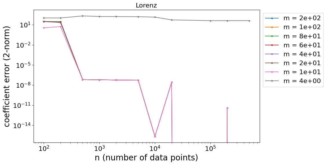
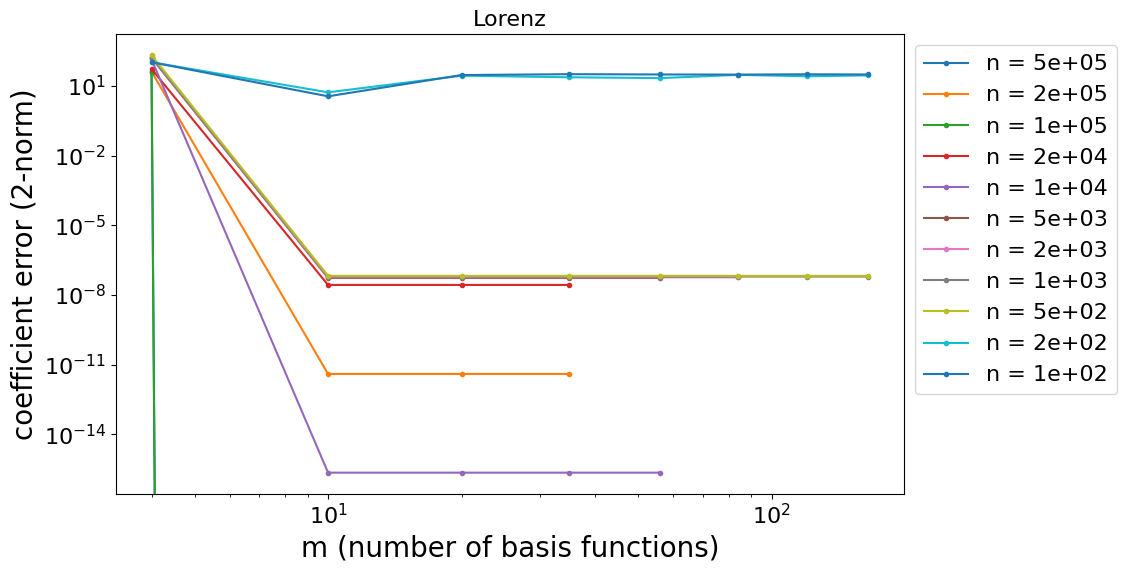
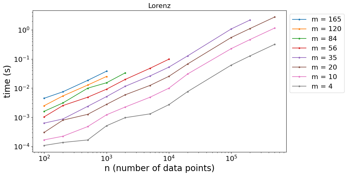
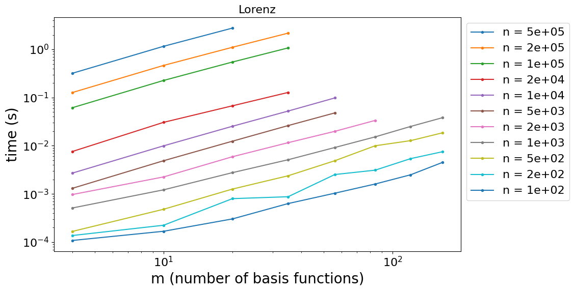
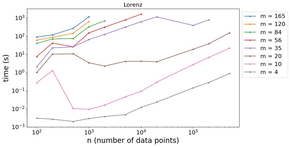
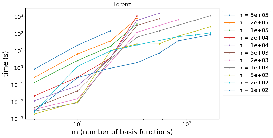
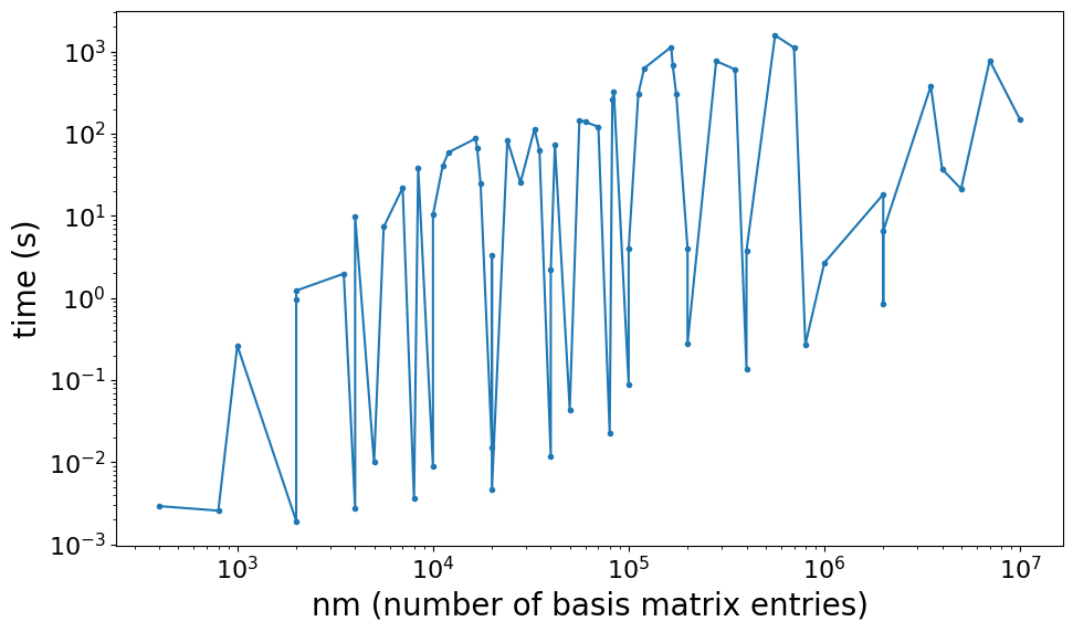
Data collected on Lorenz system by varying the number of time steps \(n\) and the number of basis functions \(m\).
Building the basis matrix is linear in \(n\), and grows with approximately \(m^{1.3}\).
Implementation overview
The basis system is below (copy/pasted from Equation 2. \[\begin{equation} \frac{d\mathbf{U}}{dt} \approx \Theta(\mathbf{U}, \mathbf{X}, t) \mathbf{c} \end{equation}\] An implementation requires the following steps:
Compute the input data \(\mathbf{U}\) (at coordinates \(\mathbf{X}\) and times \(t\)). This could be data read from a file or generated with a timestepper.
Compute the left-hand side \(\frac{d\mathbf{U}}{dt}\). This can be computed with finite differences or similar methods.
Compute the basis \(\Theta\), which requires choosing basis functions.
Compute the coefficients \(\mathbf{c}\). This can be done with any sparse regression algorithm.
Use \(\mathbf{c}\) and the basis functions to generate \(\frac{d\mathbf{U}}{dt}\) at the same data points or at new data points. (I have not done this yet).
Data generation
I’m using PETSc’s TS for Step 1. I assume a fixed-time step size and allocate memory for two arrays of Vecs to hold \(\mathbf{U}\) and \(\frac{d\mathbf{U}}{dt}\). Then in the TS’s PostStep, I record the current value of \(\mathbf{U}\). I have an option (in some examples) to either record the exact value of the derivative \(\frac{d\mathbf{U}}{dt}\) in the PostStep, or a fourth-order central difference approximation after the run is complete.
Basis computation
In order for the code to work with different \(d_u\) and \(d_x\), the computation of the basis needs to be flexible in how it reads the input data. The data for a particle moving around might be stored in a 1D Vec or a PetscScalar array, while the data for a PDE may be stored in a Vec with a DMDA. To abstract away the data access details, I set up a Variable class. An instance of the class tracks its data and knows how to access it properly. It also tracks its name for nice printouts.
From the user perspective, computing the basis simply requires defining the variables that will be present in the basis.
When the user passes these variables off to the backend, they are used to generate the basis matrix \(\Theta\). I currently have the basis matrix set up as \(d_u\) matrices as is shown in Equation 5, where each of those matrices is constant across space, as is done in Equation 7.
Coefficient computation
The previous step computes \(\Theta\), so all this step needs to do is run a sparse regression and return the results. I currently have Sequential Thresholded Least Squares implemented, with parameters specified in a SparseReg class. More backends could be tested here, and we could set sparse regression algorithm as a command-line argument.
Implementation specifics
Cross terms
I ran into an issue with the Lorenz 96 system in that it required polynomial terms of degree 2, but it contains 36 independent variables. I used Equation 3 to set up the system, meaning each variable uses the same basis matrix.
The basis function generator would originally create basis functions that had all the cross terms. In this case, that would lead to \(\binom{36 + 2}{2} = 703\) basis functions. Then the algorithm takes forever to run. In this case, we know that only nearby terms will affect each other, so I added a cross_term_range parameter, which I’ll call \(c\). For output DOF \(i\), it will only include input DOFs \(i-c,i-c+1,\ldots,i,\ldots,i+c\). So there will be a total of \(d = 2*c+1\) terms included. For \(c=2\) reduces the number of basis functions from 703 to \(\binom{d+2}{2} = \binom{7}{2} = 21\), which is much more manageable. Since each output DOF has a different set up of basis functions, this required changing from Equation 3 to Equation 5 to maintain a separate basis matrix for each output DOF.
This setup also helps the sine-cosine example. By setting the cross term range to 0, there is no intermingling of \(U_1\) and \(U_2\) in the basis functions.
For examples with coordinates (\(d_x \ne 0\)), the cross term range currently only applies to DOFs within a point. I.e., for a point’s output DOF \(i\), it will only include input DOFs \(i-c,i-c+1,\ldots,i,\ldots,i+c\) at that point.
Basis matrix generation
SINDyBasisAddVariables sets up the basis matrices. There is a separate matrix for each output DOF, so there are \(d_u\) matrices to build. Each matrix is built by looping through each basis function, and for each basis function, looping through each output coordinate and adding all \(m\) outputs to the for that coordinate. This iteration procedure generates \(\Theta'\) from Equation 7 column-wise.
Non-polynomial extraction from polynomial library
The inclusion of many non-polynomial basis functions can inflate the basis matrix \(\Theta\) to be too large. We would like to be able to use only polynomial basis functions and then post-process the results to extract the non-polynomial terms based on some polynomial expansion (e.g., Taylor series) of those terms.
Note: This section discusses a completely different problem compared to the other sections in this document, so the notation used here is completely independent of the other sections.
Subtracting out non-polynomial functions
Let \(f_j(x) = \sum_{i=0}^\infty A_{ij} x^i\) be a polynomial series representing a function, and let \(f_j^{(d)} = \sum_{i=0}^d A_{ij} x^i\) be the degree \(d\) truncation of the series. Let \(g(y) = \sum_{i=0}^d b_i y^i\) be the known function that we want to extract non-polynomial terms from. We want to express \(g(y)\) in terms of functions \(f_i(x)\), where \(y\) may be a scaled version of \(x\). \[\begin{align*} g(y) = \sum_{i=0}^d k_i y^i + \sum_{j=1}^n c_j f_j^{(d)}(\sigma_j y) \end{align*}\] We’d like to determine \(c_i\) and \(\sigma_j\). The \(k_i\) is used to absorb all the polynomials factors that aren’t represented by the sum of the non-polynomial functions. The equation can be separated into \(d+1\) equations by treating each \(y^j\) coefficient independently. \[\begin{align*} \sum_{i=0}^d b_i y^i &= \sum_{i=0}^d k_i y^i + \sum_{i=0}^d \sum_{j=1}^n A_{ij} c_j \sigma_j^i y^i \\ \implies b_i &= k_i + \sum_{j=1}^n A_{ij} c_j \sigma_j^i \,\,\,\,\, \text{ for $i \in \{0, \ldots, d\}$} \end{align*}\] This is a nonlinear problem due to the \(\sigma_j^i\) term. I’ll define \(A_{ij}' = A_{ij} \sigma^i_j\), \[\begin{align*} \mathbf{b} &= \mathbf{k} + \mathbf{A}'(\mathbf{\sigma}) \mathbf{c} \end{align*}\] We want sparsity in \(\mathbf{k}\) and \(\mathbf{c}\), which we can maybe approximate with the \(\ell_1\) norm. \[\begin{align*} &\min_{\mathbf{c},\mathbf{\sigma}} ||\mathbf{k}||_1 + ||\mathbf{c}||_1 \\& \text{subject to } \mathbf{k} = \mathbf{b} - \mathbf{A}'(\mathbf{\sigma})\mathbf{c} \end{align*}\] Or equivalently, \[\begin{align*} \min_{\mathbf{c},\mathbf{\sigma}} ||\mathbf{b} - \mathbf{A}'(\mathbf{\sigma})\mathbf{c}||_1 + ||\mathbf{c}||_1 \end{align*}\] Running this sparse optimization will show the active non-polynomial terms in \(\mathbf{c}\), although I’m not sure what a good way to run this optimization would be.
SINDy application:
Run SINDy with just polynomials and then use the above strategy to determine what non-polynomial terms are present. The coefficients for those terms can be computed as done above, or those terms can be added to the SINDy library for SINDy to be run again with the correct non-polynomial terms.
Perhaps it could be combined in the SINDy optimization, with \(\mathbf{k}\) representing the polynomial terms and \(\mathbf{c}\) representing the non-polynomial terms. \[\begin{align*} \min_{\mathbf{k},\mathbf{c},\mathbf{\sigma}} & ||\mathbf{k}||_1 + ||\mathbf{c}||_1 \\\text{subject to } \mathbf{k} &= \mathbf{b} - \mathbf{A}'(\mathbf{\sigma})\mathbf{c} \\ & \mathbf{b} = \arg \min_{\mathbf{b}'} ||\Theta \mathbf{b}' - \tfrac{d\mathbf{U}}{dt}||_2^2 + \lambda ||\mathbf{b}'||_1 \end{align*}\]
Simplification:
It will make the problem easier if the \(\sigma_j\) are assumed to be 1. Then the system becomes linear. \[\begin{align*} &\min_{\mathbf{c}} ||\mathbf{k}||_1 + ||\mathbf{c}||_1 \\& \text{subject to } \mathbf{k} = \mathbf{b} - \mathbf{A}\mathbf{c} \end{align*}\] Or equivalently, \[\begin{align*} &\min_{\mathbf{c}} \left|\left| \begin{bmatrix} \mathbf{b} \\ 0 \end{bmatrix} - \begin{bmatrix} \mathbf{A} \\ \mathbf{I}_n \end{bmatrix} \mathbf{c} \right|\right|_1 \end{align*}\] where \(\mathbf{I}_n\) is the identity. In this case, we can think of this optimization as simply expressing the original coefficients \(\mathbf{b} \in \mathbb{R}^d\) in a new basis \(\mathbf{B} \in \mathbb{R}^{d \times (n+d)}\), which is composed of the original polynomial basis, plus extra functions. Then we want to find the set of coefficients \(\mathbf{c}' \in \mathbb{R}^(d+n)\), such that \(\mathbf{b} = \mathbf{B} \mathbf{c'}\) and \(\mathbf{c'}\) is as sparse as possible. Using the notation from above, the variables are defined as follows, \[\begin{align*} \mathbf{c}' &= \begin{bmatrix} \mathbf{k} \\ \mathbf{c} \end{bmatrix} \\ \mathbf{B} &= \begin{bmatrix} \mathbf{I}_d & \mathbf{A} \end{bmatrix} \end{align*}\]
Factoring out non-polynomial functions
The above formulation handles cases where \(g(y)\) is equal to a polynomial plus some non-polynomial terms, where the non-polynomial terms have to be specified in advance (e.g., sine, cosine, the exponential function). But there may be terms like \(x \sin(x)\) or \(x\sin x + x^3\sin x\), where a polynomial is multiplied by a non-polynomial. These could be included as basis functions, but if we can extract them automatically, it will make the basis library more tractable. Consider a function that is multiplied by a monomial of degree \(r \le d_r\). (The previous section is equivalent to \(d_r=0\). This section essentially augments the non-polynomial library with the product of polynomials with the non-polynomials). \[\begin{align*} x^r f_j(x) = \sum_{i=0}^\infty A_{ij} x^{r+i} = \sum_{i=r}^\infty A_{i-r,j} x^{i} \end{align*}\]
Again, let \(g(y) = \sum_{i=0}^d b_i y^i\) be the known function that we want to extract non-polynomial terms from. We want to express \(g(y)\) in terms of functions \(f_i(x)\) multiplied by monomials. \[\begin{align*} g(y) &= \sum_{i=0}^d k_i y^i + \sum_{j=1}^n \sum_{r=0}^{d_r} c_{jr} y^r f_j^{(d)}(\sigma_j y) \\ &= \sum_{i=0}^d k_i y^i + \sum_{j=1}^n \sum_{r=0}^{d_r} c_{jr} \sigma_j^{-r} x^r f_j^{(d)}(\sigma_j y) \end{align*}\] \[\begin{align*} \sum_{i=0}^d b_i y^i &= \sum_{i=0}^d k_i y^i + \sum_{j=1}^n \sum_{r=0}^{d_r} \sum_{i=r}^d A_{i-r,j} c_{jr} \sigma_j^{i-r} y^i \\ \sum_{i=0}^d b_i y^i &= \sum_{i=0}^d k_i y^i + \sum_{j=1}^n \sum_{i=0}^d \sum_{r=1}^{\min(i,d_r)} A_{i-r,j} c_{jr} \sigma_j^{i-r} y^i \\ \implies b_i &= k_i + \sum_{j=1}^n \sum_{r=1}^{\min(i,d_r)} A_{i-r,j} \sigma_j^{i-r} c_{jr} \,\,\,\,\, \text{ for $i \in \{0, \ldots, d\}$} \end{align*}\] Linearize \(c_{jr}\) by treating \(jr\) as a single index that goes from 1 to \(nd_r\), and let the matrix \(\mathbf{A}' \in \mathbb{R}^{d \times nd_r}\) be defined as \(A_{i,jr}' = A_{i-r,j}\sigma_j^{i-r}\). This yields the same form as the previous section. \[\begin{align*} \mathbf{b} &= \mathbf{k} + \mathbf{A}'(\mathbf{\sigma}) \mathbf{c} \end{align*}\] We want sparsity in \(\mathbf{k}\) and \(\mathbf{c}\), which we can maybe approximate with the \(\ell_1\) norm, although this optimization may not work. \[\begin{align*} &\min_{\mathbf{c},\mathbf{\sigma}} ||\mathbf{k}||_1 + ||\mathbf{c}||_1 \\& \text{subject to } \mathbf{k} = \mathbf{b} - \mathbf{A}'(\mathbf{\sigma})\mathbf{c} \end{align*}\]
One-at-a-time algorithm
The optimization problem above may be too difficult. An alternative method is to extract one non-polynomial function at a time. This can be repeated for any desired non-polynomial function.
Again, let \(g(y) = \sum_{i=0}^d b_i y^i\) be the known function that we want to extract non-polynomial terms from. We want to express \(g(y)\) in terms of functions \(f(x)\) multiplied by monomials, plus a polynomial function \(h\). Assume we have a truncated series expansion of \(f\) in terms of polynomials. \[\begin{align*} g(y) &= h(y) + c f^{(d)}(\sigma y) \\ \sum_{i=0}^d b_i y^i &= \sum_{i=0}^d k_i y^i + \sum_{i=0}^d c a_i \sigma^i x^i \\ \implies b_i &= k_i + c a_i \sigma^i \\ \implies \mathbf{b} &= \mathbf{k} + c D(\sigma) \mathbf{a} \\ D(\sigma) &= \text{diag}(1, \sigma, \sigma^2, \ldots, \sigma^d) \end{align*}\] We want to choose \(c\) and \(\sigma\) such that they zero out at least one term in \(\mathbf{k}\). Since we’re choosing two parameters, though, we’ll be able to zero out two terms. A direct algorithm would do the following:
For any two entries \(i,j\) in \(\mathbf{k}\), with \(i < j\):
Skip this \(i,j\) pair if \(a_i a_j b_i b_j = 0\), which means one of the terms doesn’t show up in \(g\), so zeroing this term out leads to \(c = 0\), or it means one of the terms doesn’t show up in \(f\), so we can’t use it zero out terms in \(g\).
Solve for \(c\) and \(\sigma\) to make these two entries 0. \[\begin{equation*} \sigma = \left(\frac{a_i b_j}{a_j b_i} \right)^{\frac{1}{j-i}} \text{ and } c = \frac{b_i}{a_i\sigma^i} \end{equation*}\]
Record a measure of the sparsity of \(\mathbf{k}\).
Choose the \(c\) and \(\sigma\) that lead to the best sparsity of \(\mathbf{k}\), or choose them to be zero if the sparsity of \(\mathbf{b}\) is better.
One this function is extracted, the algorithm can be repeated for a different function. Determining the optimal extractions for a library of non-polynomial functions may be a combinatorially large problem.